
Tutorial
The field of theoretical quantum physics is notoriously difficult to grasp, and information about it is often obfuscated in complex rhetoric. Leave that behind with
DMRGenie!
DMRGenie is intended to be a tool for research and education.
Learn how to use its cutting edge features with this guide.
To get up to speed on
Tensor Networks check out these papers:
- "Méthodes de calcul avec réseaux de tenseurs (Basic tensor network computations in physics)" by T.E. Baker, S. Desrosiers, M. Tremblay, and M.P. Thompson, which includes both a French and English version.
- "The basics of tensor networks: An overview of tensors and renormalization" by S. Desrosiers, G.B. Evenbly, and T.E. Baker, a short paper on the fundamentals of tensor network algorithms.
Algorithm Runner
The
Algorithm Runner allows you to run known tensor network algorithms without coding knowledge. Currently, the density matrix renormalization group (DMRG) algorithm is the only one available, but more are coming soon.
DMRG
This tutorial will guide you through running DMRG on known and custom models. Let's start by going over the basics of what everything means.
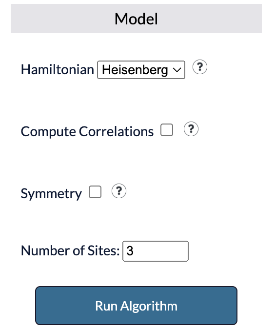
On the
Algorithm Runner page you will be met with the following option menu. Each option is as follows:
- Hamiltonian: The model which DMRG will be run on in Matrix Product Operator (MPO) form.
- Compute Correlations: Specify operators to be evaluated at each lattice site to receive tensors populated with correlation functions upon computation.
- Symmetry: Enforce quantum symmetries. Selecting this will run DMRG on a separate quantum model as well.
- Number of Sites: MPO terms, with a maximum of 15 allowed.
With the default options set, clicking
Run Algorithm will run DMRG on the given model and the ground state energy will be given, as well as any other specified outputs.
Hamiltonians
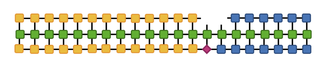
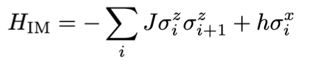
The 1-dimensional Ising spin model represents a system of particles with nearest-neighbour interactions along a line. A simple version of it can be expressed
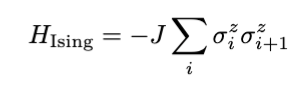 where J is the coupling constant. A magnetic field can be imposed by adding the term with constant h, representing magnetic field strength,
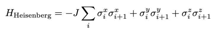
 The 1-dimensional Ising model shares some resemblance to the Heisenberg model, which can be expressed
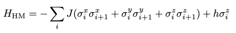
 A magnetic field term can similarly be added on
There are three built in models one can select from:
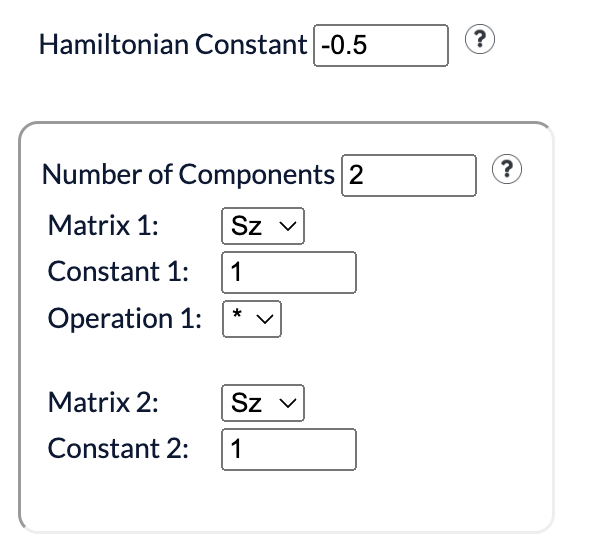
The 1-dimensional Ising model with a coupling constant of J=0.5 can be input as
Then an external magnetic field with constants J=0.5 and h=0.05 can be imposed as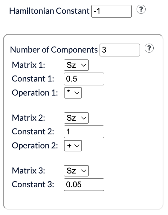
Then for the Heisenberg model with J = 0.5 the input would be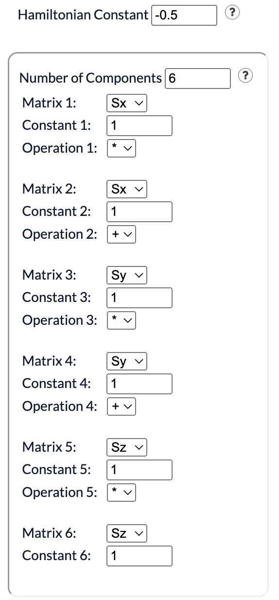
where J is the coupling constant. A magnetic field can be imposed by adding the term with constant h, representing magnetic field strength,
The 1-dimensional Ising model shares some resemblance to the Heisenberg model, which can be expressed
A magnetic field term can similarly be added on
There are three built in models one can select from:
- Heisenberg model
- Hubbard model
- t-J model
Constructing Custom Hamiltonians
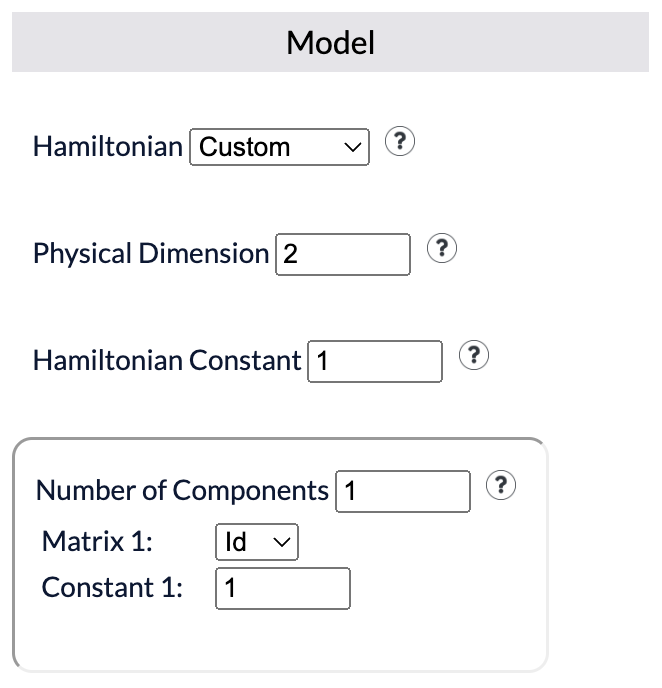
Custom Hamiltonians can be specified and constructed as well. Let's consider the Hamiltonian of the 1-dimensional Ising model. Begin construction by selecting Hamiltonian -> Custom
- Physical dimension: The dimension of the outward facing indices of MPO terms.
- Hamiltonian constant: Multiplicative constant applied to Hamiltonian sum.
- Components: Operators specified in Hamiltonian.
Then an external magnetic field with constants J=0.5 and h=0.05 can be imposed as
Then for the Heisenberg model with J = 0.5 the input would be
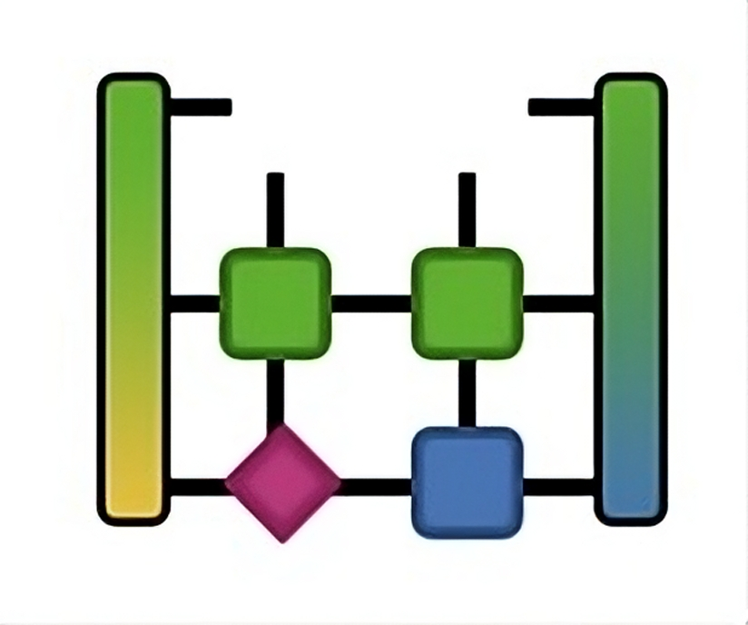
Tensor Network Builder
The
Tensor Network Builder allows you to craft novel tensor network algorithms and test your ideas. Effortlessly connect, contract, and decompose tensors on the canvas in seconds!

The process boils down into two parts:
- Specify all the steps by placing, contracting, and decomposing tensors.
- Submit the steps to be run with TensorPACK and receive the output.
Operations
Below outlines how to apply each operation and then run the set of steps to obtain an output.
Creating a Tensor
Tensors are created under the Drag and Drop section of the options menu. The rank of the tensor can be specified before the tensor is created. The rank can be from 0 and 4. Tensors made this was are initialized as random unitaries.
Uploading a Tensor
Tensors can also be uploaded as well. To do this, index names and their corresponding dimensions must be provided. If the sizes are incorrect, then contraction will fail or give undesired results. Only text files are accepted, and their contents must be in Julia array syntax where one set of square braces encloses the tensor elements and semicolons are used to differentiate between indices (e.g. columns). This is the same syntax convention as output tensors are written in.
For example, a 2 by 3 tensor should be input as
Or a 2 by 5 by 3 tensor should be input as
Or a 2 by 3 by 4 by 5 tensor should be input as
Code such as
For example, a 2 by 3 tensor should be input as
[6 1 2; 6 4 7]
Or a 2 by 5 by 3 tensor should be input as
[9 7 1 9 8; 6 4 4 9 6;;;
3 5 6 9 8; 4 6 3 9 1;;;
7 3 3 5 9; 2 4 8 5 8]
Or a 2 by 3 by 4 by 5 tensor should be input as
[8 3 9; 5 3 2;;; 5 9 5; 9 8 4;;; 2 7 7; 6 4 3;;;;
7 1 1; 7 8 4;;; 2 2 3; 3 3 5;;; 6 1 1; 7 6 2;;;;
3 6 7; 8 6 6;;; 4 9 9; 1 9 7;;; 8 4 1; 3 7 2;;;;
5 9 9; 4 6 5;;; 2 7 7; 7 2 5;;; 9 2 3; 8 9 8]
Code such as
println(rand(2, 3, 4)) should produce tensors of this format by default.
Connecting Tensors
Tensors can be connected by dragging between the points on any two tensors. However, there is a maximum of one connection per point. A free index can be created by dragging from a connection point to the network canvas.
Contract
The Contract option accepts two tensor IDs and contracts them into one. Tensors can be contracted if they are connected to each other by an edge, or if each has a free index with a common name and dimension. If there are no common indices between two tensors then they cannot be contracted.
Singular Value Decomposition (SVD)
The SVD option accepts the ID of a tensor and the desired grouping of indices. The operation will decompose tensor A as A = UDV, where D is a diagonal matrix and U and V are unitaries. The resulting tensors will be labelled accordingly.
QR and LQ Decompositions
The QR decomposition accepts the ID of a tensor and the desired grouping of indices. The operation will decompose A as A = QR, where Q is orthogonal and R is an upper triangular when reshaped into a matrix.
The LQ decomposition is similar, except it decomposes as A = LQ where L is lower triangular when reshaped as a matrix.
The LQ decomposition is similar, except it decomposes as A = LQ where L is lower triangular when reshaped as a matrix.
Eigenvalue Decomposition
The Eigenvalue decomposition accepts just the ID of a tensor. The tensor must be able to be reshaped into a square matrix. The result of the operation will result in a tensor of eigenvectors, its dual, and a diagonal tensor of eigenvalues.
Split Index and Connect Index
Split Index accepts the name of an index. If two tensors are connected, then the connection will be turned into a free index for each tensor.
Connect Index accepts the name of two indices and connects them directly. The dimensions of the indices must match.
Connect Index accepts the name of two indices and connects them directly. The dimensions of the indices must match.
Run Network Steps
All the steps for the network will be run and the tensors resulting from the final step will be given in Julia array syntax in a text downloadable file.